Exercise 8.10
import pandas as pd
import numpy as np
import matplotlib.pyplot as plt
from sklearn.ensemble import GradientBoostingRegressor
from sklearn.metrics import mean_squared_error
from sklearn.linear_model import LinearRegression
from sklearn.linear_model import LassoCV
from sklearn.ensemble import BaggingRegressor

%matplotlib inline
df = pd.read_csv('../data/Hitters.csv', index_col=0)
df.head()
| AtBat | Hits | HmRun | Runs | RBI | Walks | Years | CAtBat | CHits | CHmRun | CRuns | CRBI | CWalks | League | Division | PutOuts | Assists | Errors | Salary | NewLeague | |
|---|---|---|---|---|---|---|---|---|---|---|---|---|---|---|---|---|---|---|---|---|
| -Andy Allanson | 293 | 66 | 1 | 30 | 29 | 14 | 1 | 293 | 66 | 1 | 30 | 29 | 14 | A | E | 446 | 33 | 20 | NaN | A |
| -Alan Ashby | 315 | 81 | 7 | 24 | 38 | 39 | 14 | 3449 | 835 | 69 | 321 | 414 | 375 | N | W | 632 | 43 | 10 | 475.0 | N |
| -Alvin Davis | 479 | 130 | 18 | 66 | 72 | 76 | 3 | 1624 | 457 | 63 | 224 | 266 | 263 | A | W | 880 | 82 | 14 | 480.0 | A |
| -Andre Dawson | 496 | 141 | 20 | 65 | 78 | 37 | 11 | 5628 | 1575 | 225 | 828 | 838 | 354 | N | E | 200 | 11 | 3 | 500.0 | N |
| -Andres Galarraga | 321 | 87 | 10 | 39 | 42 | 30 | 2 | 396 | 101 | 12 | 48 | 46 | 33 | N | E | 805 | 40 | 4 | 91.5 | N |
df = pd.get_dummies(df)
df.head()
| AtBat | Hits | HmRun | Runs | RBI | Walks | Years | CAtBat | CHits | CHmRun | ... | PutOuts | Assists | Errors | Salary | League_A | League_N | Division_E | Division_W | NewLeague_A | NewLeague_N | |
|---|---|---|---|---|---|---|---|---|---|---|---|---|---|---|---|---|---|---|---|---|---|
| -Andy Allanson | 293 | 66 | 1 | 30 | 29 | 14 | 1 | 293 | 66 | 1 | ... | 446 | 33 | 20 | NaN | 1.0 | 0.0 | 1.0 | 0.0 | 1.0 | 0.0 |
| -Alan Ashby | 315 | 81 | 7 | 24 | 38 | 39 | 14 | 3449 | 835 | 69 | ... | 632 | 43 | 10 | 475.0 | 0.0 | 1.0 | 0.0 | 1.0 | 0.0 | 1.0 |
| -Alvin Davis | 479 | 130 | 18 | 66 | 72 | 76 | 3 | 1624 | 457 | 63 | ... | 880 | 82 | 14 | 480.0 | 1.0 | 0.0 | 0.0 | 1.0 | 1.0 | 0.0 |
| -Andre Dawson | 496 | 141 | 20 | 65 | 78 | 37 | 11 | 5628 | 1575 | 225 | ... | 200 | 11 | 3 | 500.0 | 0.0 | 1.0 | 1.0 | 0.0 | 0.0 | 1.0 |
| -Andres Galarraga | 321 | 87 | 10 | 39 | 42 | 30 | 2 | 396 | 101 | 12 | ... | 805 | 40 | 4 | 91.5 | 0.0 | 1.0 | 1.0 | 0.0 | 0.0 | 1.0 |
5 rows × 23 columns
(a)
# Remove observations for whom the salary information is unknown.
df = df.dropna(subset=['Salary'])
# Log transform salaries
df['Salary'] = np.log(df['Salary'])
(b)
# Create training and testing
# We don't use the train_test_split because we don't want to split data randomly.
X = df.drop(['Salary'], axis=1)
y = df['Salary']

X_train = X.ix[:200,:]
y_train = y.ix[:200]
X_test = X.ix[200:,:]
y_test = y.ix[200:]
(c)
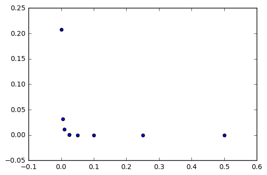
# Boosting with different shrinkage values
shrinkage_values = [.001, .025, .005, .01, .025, .05, .1, .25, .5]
mses = []
for i in shrinkage_values:
    bst = GradientBoostingRegressor(learning_rate=i, n_estimators=1000, random_state=1)
    bst.fit(X_train, y_train)
    mses.append(mean_squared_error(y_train, bst.predict(X_train)))
# Plot training set MSE for different shrinkage values
plt.scatter(shrinkage_values, mses)
<matplotlib.collections.PathCollection at 0xf98e0f0>
(d)
# Boosting with different shrinkage values
shrinkage_values = [.001, .025, .005, .01, .025, .05, .1, .25, .5]
mses = []
for i in shrinkage_values:
    bst = GradientBoostingRegressor(learning_rate=i, n_estimators=1000, random_state=1)
    bst.fit(X_train, y_train)
    mses.append(mean_squared_error(y_test, bst.predict(X_test)))
# Plot training set MSE for different shrinkage values
plt.scatter(shrinkage_values, mses)
<matplotlib.collections.PathCollection at 0xf9f5240>
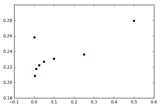
# Get minimum test MSE value
print('Minimum test MSE:', np.min(mses))
Minimum test MSE: 0.208753925111
# Index of the shrinkage_value that leads to the minimum test MSE
np.where(mses == np.min(mses))
(array([2], dtype=int64),)
(e)
# Linear regression
rgr = LinearRegression()
rgr.fit(X_train, y_train)

print('Minimum test MSE:', mean_squared_error(y_test, rgr.predict(X_test)))
Minimum test MSE: 0.491795937545
# Cross-validated lasso
lasso = LassoCV(cv=5)
lasso.fit(X_train, y_train)

print('Minimum test MSE:', mean_squared_error(y_test, lasso.predict(X_test)))
Minimum test MSE: 0.486586369603
The test MSE obtained using boosting is lower than the test MSE obtained using a linear regression or a lasso regularized regression. This means that, according to this error metric, boosting is the model with better predictive capacity.
(f)
# Plot features importance to understand their importance.
bst = GradientBoostingRegressor(learning_rate=0.005)  # 0.005 is the learning_rate corresponding to the best test MSE
bst.fit(X_train, y_train)

feature_importance = bst.feature_importances_*100
rel_imp = pd.Series(feature_importance, index=X.columns).sort_values(inplace=False)
rel_imp.T.plot(kind='barh', color='r')
plt.xlabel('Variable importance')
<matplotlib.text.Text at 0xd682e10>
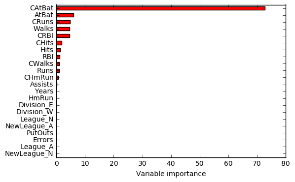
According to the figure, the most important predictors seem to be: CAtBat, AtBat, CRuns, Walks and CRBI.
(g)
# Fit bagging regressor
bagging = BaggingRegressor()
bagging.fit(X_train, y_train)
BaggingRegressor(base_estimator=None, bootstrap=True,
         bootstrap_features=False, max_features=1.0, max_samples=1.0,
         n_estimators=10, n_jobs=1, oob_score=False, random_state=None,
         verbose=0, warm_start=False)
# Test MSE
print('Test MSE:', mean_squared_error(y_test, bagging.predict(X_test)))
Test MSE: 0.253358375264