Exercise 2.10
%matplotlib inline

import pandas as pd
import seaborn as sns
import numpy as np
import matplotlib.pyplot as plt
a) Dataset overview
In Python we can load the Boston dataset using scikit-learn.
from sklearn.datasets import load_boston

boston = load_boston()
df = pd.DataFrame(boston.data, columns=boston.feature_names)
df['target'] = boston.target
print(boston['DESCR'])
Boston House Prices dataset
===========================

Notes
------
Data Set Characteristics:

    :Number of Instances: 506

    :Number of Attributes: 13 numeric/categorical predictive

    :Median Value (attribute 14) is usually the target

    :Attribute Information (in order):
        - CRIM     per capita crime rate by town
        - ZN       proportion of residential land zoned for lots over 25,000 sq.ft.
        - INDUS    proportion of non-retail business acres per town
        - CHAS     Charles River dummy variable (= 1 if tract bounds river; 0 otherwise)
        - NOX      nitric oxides concentration (parts per 10 million)
        - RM       average number of rooms per dwelling
        - AGE      proportion of owner-occupied units built prior to 1940
        - DIS      weighted distances to five Boston employment centres
        - RAD      index of accessibility to radial highways
        - TAX      full-value property-tax rate per $10,000
        - PTRATIO  pupil-teacher ratio by town
        - B        1000(Bk - 0.63)^2 where Bk is the proportion of blacks by town
        - LSTAT    % lower status of the population
        - MEDV     Median value of owner-occupied homes in $1000's

    :Missing Attribute Values: None

    :Creator: Harrison, D. and Rubinfeld, D.L.

This is a copy of UCI ML housing dataset.
http://archive.ics.uci.edu/ml/datasets/Housing


This dataset was taken from the StatLib library which is maintained at Carnegie Mellon University.

The Boston house-price data of Harrison, D. and Rubinfeld, D.L. 'Hedonic
prices and the demand for clean air', J. Environ. Economics & Management,
vol.5, 81-102, 1978.   Used in Belsley, Kuh & Welsch, 'Regression diagnostics
...', Wiley, 1980.   N.B. Various transformations are used in the table on
pages 244-261 of the latter.

The Boston house-price data has been used in many machine learning papers that address regression
problems.

**References**

   - Belsley, Kuh & Welsch, 'Regression diagnostics: Identifying Influential Data and Sources of Collinearity', Wiley, 1980. 244-261.
   - Quinlan,R. (1993). Combining Instance-Based and Model-Based Learning. In Proceedings on the Tenth International Conference of Machine Learning, 236-243, University of Massachusetts, Amherst. Morgan Kaufmann.
   - many more! (see http://archive.ics.uci.edu/ml/datasets/Housing)
df.head()
| CRIM | ZN | INDUS | CHAS | NOX | RM | AGE | DIS | RAD | TAX | PTRATIO | B | LSTAT | target | |
|---|---|---|---|---|---|---|---|---|---|---|---|---|---|---|
| 0 | 0.00632 | 18.0 | 2.31 | 0.0 | 0.538 | 6.575 | 65.2 | 4.0900 | 1.0 | 296.0 | 15.3 | 396.90 | 4.98 | 24.0 |
| 1 | 0.02731 | 0.0 | 7.07 | 0.0 | 0.469 | 6.421 | 78.9 | 4.9671 | 2.0 | 242.0 | 17.8 | 396.90 | 9.14 | 21.6 |
| 2 | 0.02729 | 0.0 | 7.07 | 0.0 | 0.469 | 7.185 | 61.1 | 4.9671 | 2.0 | 242.0 | 17.8 | 392.83 | 4.03 | 34.7 |
| 3 | 0.03237 | 0.0 | 2.18 | 0.0 | 0.458 | 6.998 | 45.8 | 6.0622 | 3.0 | 222.0 | 18.7 | 394.63 | 2.94 | 33.4 |
| 4 | 0.06905 | 0.0 | 2.18 | 0.0 | 0.458 | 7.147 | 54.2 | 6.0622 | 3.0 | 222.0 | 18.7 | 396.90 | 5.33 | 36.2 |
np.shape(df)
(506, 14)
Number of rows and columns 506 rows. 14 columns.
Rows and columns description Each rows is town in Boston area. Columns are features that can influence house price such as per capita crime rate by town ('CRIM').
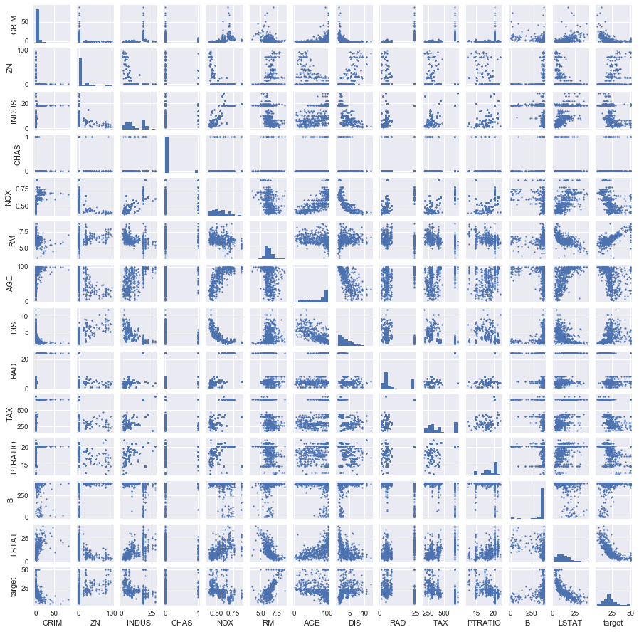
b) Scatterplots
- We'll use seaborn to get a quick overview of pairwise relationships
g = sns.PairGrid(df)
g.map_upper(plt.scatter, s=3)
g.map_diag(plt.hist)
g.map_lower(plt.scatter, s=3)
g.fig.set_size_inches(12, 12)
plt.scatter(df['RM'], df['target'])
plt.xlabel('RM')
plt.ylabel('target');
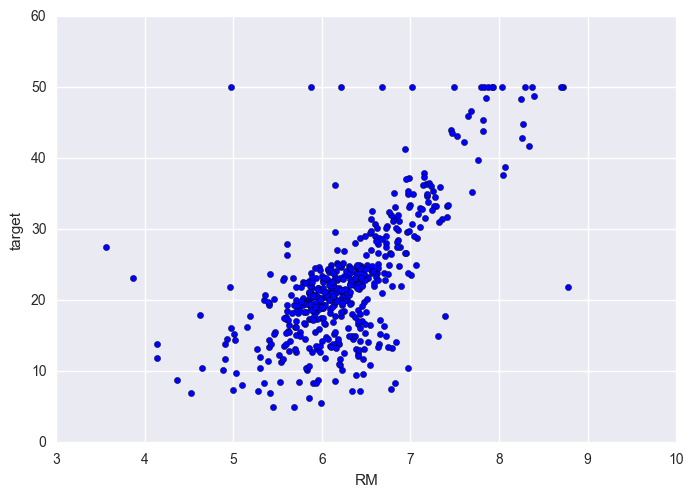
Findings It seems to exist a positive linear relationship between RM and target This is expected as RM is the number of rooms (more space, higher price)
plt.scatter(df['LSTAT'], df['target'])
plt.xlabel('LSTAT')
plt.ylabel('target');
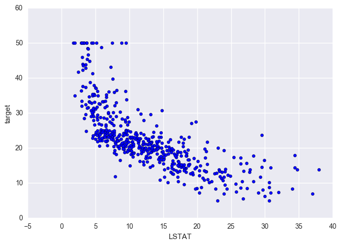
Findings LSTAT and target seem to have a negative non-linear relationship This is expected as LSTAT is the percent of lower status people (lower status, lower incomes, cheaper houses)
plt.scatter(df['RM'], df['LSTAT'])
plt.xlabel('RM')
plt.ylabel('LSTAT');
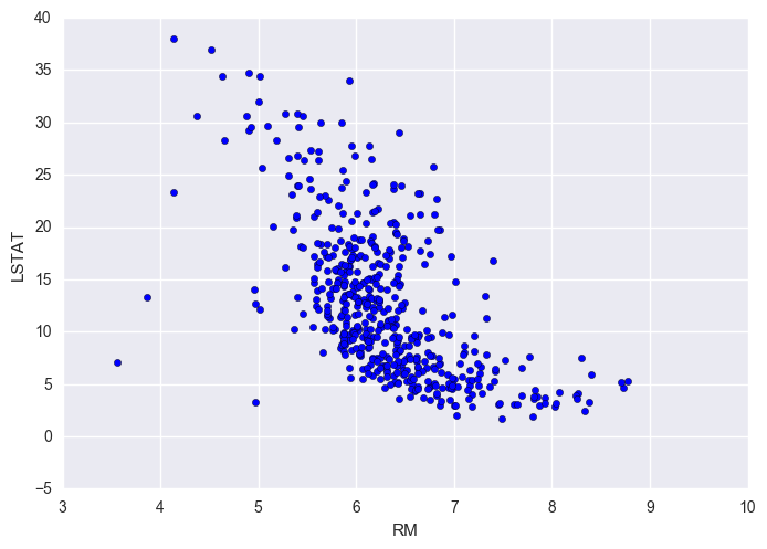
Findings It seems to exist a negative non-linear relationship between LSTAT and RM It makes sense since people with less money (higher LSTAT) can't afford bigger houses (high RM)
c) Predictors associated with capita crime rate
df.corrwith(df['CRIM']).sort_values()
target    -0.385832
DIS       -0.377904
B         -0.377365
RM        -0.219940
ZN        -0.199458
CHAS      -0.055295
PTRATIO    0.288250
AGE        0.350784
INDUS      0.404471
NOX        0.417521
LSTAT      0.452220
TAX        0.579564
RAD        0.622029
CRIM       1.000000
dtype: float64
Looking at the previous scatterplots and the correlation of each variable with 'CRIM', we will have a closer at the 3 with the largest correlation, namely: RAD, index of accessibility to radial highways, TAX, full-value property-tax rate (in dollars per $10,000), * LSTAT, percentage of lower status of the population.
ax = sns.boxplot(x="RAD", y="CRIM", data=df)
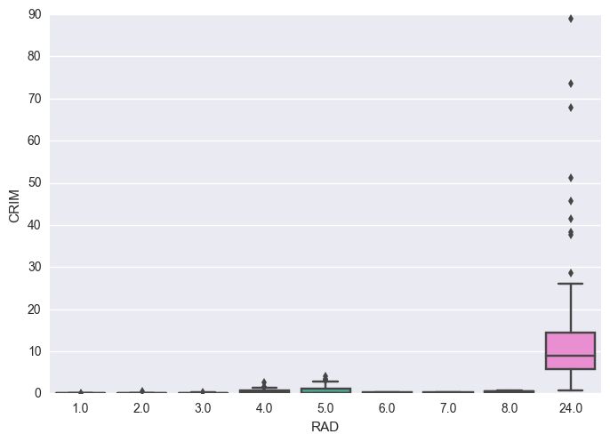
Findings * When RAD is equal to 24 (its highest value), average CRIM is much higher and CRIM range is much larger.
plt.scatter(df['TAX'], df['CRIM'])
plt.xlabel('TAX')
plt.ylabel('CRIM');
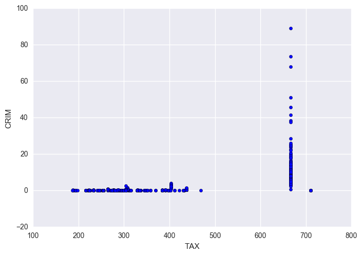
Findings * When TAX is equal to 666, average CRIM is much higher and CRIM range is much larger.
plt.scatter(df['LSTAT'], df['CRIM'])
plt.xlabel('LSTAT')
plt.ylabel('CRIM');
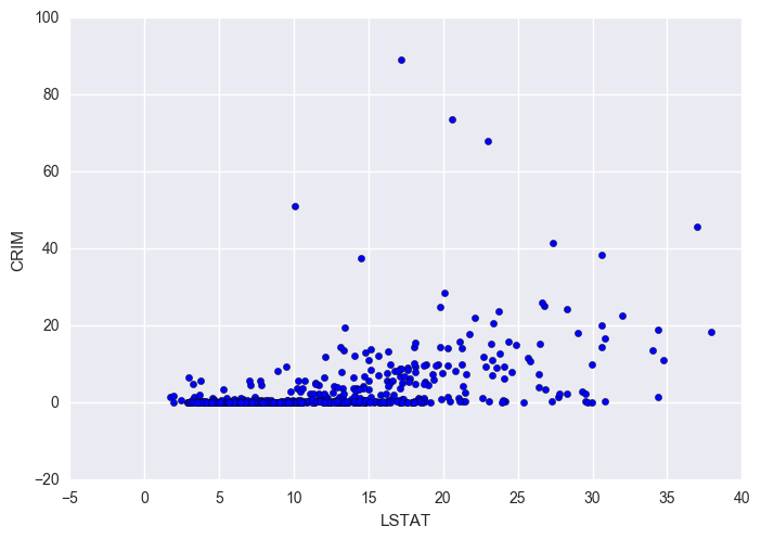
Findings For lower values of LSTAT (< 10), CRIM is always under 10. For LSTAT > 10, there is a wider spread of CRIM. For LSTAT < 20, a large proportion of the data points is very close to CRIM = 0.
d) Crime rate, tax rate and pupil-teacher ratio in suburbs
df.ix[df['CRIM'].nlargest(5).index]
| CRIM | ZN | INDUS | CHAS | NOX | RM | AGE | DIS | RAD | TAX | PTRATIO | B | LSTAT | target | |
|---|---|---|---|---|---|---|---|---|---|---|---|---|---|---|
| 380 | 88.9762 | 0.0 | 18.1 | 0.0 | 0.671 | 6.968 | 91.9 | 1.4165 | 24.0 | 666.0 | 20.2 | 396.90 | 17.21 | 10.4 |
| 418 | 73.5341 | 0.0 | 18.1 | 0.0 | 0.679 | 5.957 | 100.0 | 1.8026 | 24.0 | 666.0 | 20.2 | 16.45 | 20.62 | 8.8 |
| 405 | 67.9208 | 0.0 | 18.1 | 0.0 | 0.693 | 5.683 | 100.0 | 1.4254 | 24.0 | 666.0 | 20.2 | 384.97 | 22.98 | 5.0 |
| 410 | 51.1358 | 0.0 | 18.1 | 0.0 | 0.597 | 5.757 | 100.0 | 1.4130 | 24.0 | 666.0 | 20.2 | 2.60 | 10.11 | 15.0 |
| 414 | 45.7461 | 0.0 | 18.1 | 0.0 | 0.693 | 4.519 | 100.0 | 1.6582 | 24.0 | 666.0 | 20.2 | 88.27 | 36.98 | 7.0 |
df.ix[df['TAX'].nlargest(5).index]
| CRIM | ZN | INDUS | CHAS | NOX | RM | AGE | DIS | RAD | TAX | PTRATIO | B | LSTAT | target | |
|---|---|---|---|---|---|---|---|---|---|---|---|---|---|---|
| 488 | 0.15086 | 0.0 | 27.74 | 0.0 | 0.609 | 5.454 | 92.7 | 1.8209 | 4.0 | 711.0 | 20.1 | 395.09 | 18.06 | 15.2 |
| 489 | 0.18337 | 0.0 | 27.74 | 0.0 | 0.609 | 5.414 | 98.3 | 1.7554 | 4.0 | 711.0 | 20.1 | 344.05 | 23.97 | 7.0 |
| 490 | 0.20746 | 0.0 | 27.74 | 0.0 | 0.609 | 5.093 | 98.0 | 1.8226 | 4.0 | 711.0 | 20.1 | 318.43 | 29.68 | 8.1 |
| 491 | 0.10574 | 0.0 | 27.74 | 0.0 | 0.609 | 5.983 | 98.8 | 1.8681 | 4.0 | 711.0 | 20.1 | 390.11 | 18.07 | 13.6 |
| 492 | 0.11132 | 0.0 | 27.74 | 0.0 | 0.609 | 5.983 | 83.5 | 2.1099 | 4.0 | 711.0 | 20.1 | 396.90 | 13.35 | 20.1 |
df.ix[df['PTRATIO'].nlargest(5).index]
| CRIM | ZN | INDUS | CHAS | NOX | RM | AGE | DIS | RAD | TAX | PTRATIO | B | LSTAT | target | |
|---|---|---|---|---|---|---|---|---|---|---|---|---|---|---|
| 354 | 0.04301 | 80.0 | 1.91 | 0.0 | 0.413 | 5.663 | 21.9 | 10.5857 | 4.0 | 334.0 | 22.0 | 382.80 | 8.05 | 18.2 |
| 355 | 0.10659 | 80.0 | 1.91 | 0.0 | 0.413 | 5.936 | 19.5 | 10.5857 | 4.0 | 334.0 | 22.0 | 376.04 | 5.57 | 20.6 |
| 127 | 0.25915 | 0.0 | 21.89 | 0.0 | 0.624 | 5.693 | 96.0 | 1.7883 | 4.0 | 437.0 | 21.2 | 392.11 | 17.19 | 16.2 |
| 128 | 0.32543 | 0.0 | 21.89 | 0.0 | 0.624 | 6.431 | 98.8 | 1.8125 | 4.0 | 437.0 | 21.2 | 396.90 | 15.39 | 18.0 |
| 129 | 0.88125 | 0.0 | 21.89 | 0.0 | 0.624 | 5.637 | 94.7 | 1.9799 | 4.0 | 437.0 | 21.2 | 396.90 | 18.34 | 14.3 |
df.describe()
| CRIM | ZN | INDUS | CHAS | NOX | RM | AGE | DIS | RAD | TAX | PTRATIO | B | LSTAT | target | |
|---|---|---|---|---|---|---|---|---|---|---|---|---|---|---|
| count | 506.000000 | 506.000000 | 506.000000 | 506.000000 | 506.000000 | 506.000000 | 506.000000 | 506.000000 | 506.000000 | 506.000000 | 506.000000 | 506.000000 | 506.000000 | 506.000000 |
| mean | 3.593761 | 11.363636 | 11.136779 | 0.069170 | 0.554695 | 6.284634 | 68.574901 | 3.795043 | 9.549407 | 408.237154 | 18.455534 | 356.674032 | 12.653063 | 22.532806 |
| std | 8.596783 | 23.322453 | 6.860353 | 0.253994 | 0.115878 | 0.702617 | 28.148861 | 2.105710 | 8.707259 | 168.537116 | 2.164946 | 91.294864 | 7.141062 | 9.197104 |
| min | 0.006320 | 0.000000 | 0.460000 | 0.000000 | 0.385000 | 3.561000 | 2.900000 | 1.129600 | 1.000000 | 187.000000 | 12.600000 | 0.320000 | 1.730000 | 5.000000 |
| 25% | 0.082045 | 0.000000 | 5.190000 | 0.000000 | 0.449000 | 5.885500 | 45.025000 | 2.100175 | 4.000000 | 279.000000 | 17.400000 | 375.377500 | 6.950000 | 17.025000 |
| 50% | 0.256510 | 0.000000 | 9.690000 | 0.000000 | 0.538000 | 6.208500 | 77.500000 | 3.207450 | 5.000000 | 330.000000 | 19.050000 | 391.440000 | 11.360000 | 21.200000 |
| 75% | 3.647423 | 12.500000 | 18.100000 | 0.000000 | 0.624000 | 6.623500 | 94.075000 | 5.188425 | 24.000000 | 666.000000 | 20.200000 | 396.225000 | 16.955000 | 25.000000 |
| max | 88.976200 | 100.000000 | 27.740000 | 1.000000 | 0.871000 | 8.780000 | 100.000000 | 12.126500 | 24.000000 | 711.000000 | 22.000000 | 396.900000 | 37.970000 | 50.000000 |
Findings The 5 towns shown in CRIM table are particularly high All the towns shown in the TAX table have maximum TAX level * PTRATIO table shows towns with high pupil-teacher ratios but not so uneven
e) Suburbs bounding the Charles river
df['CHAS'].value_counts()[1]
35
(f) Median pupil-teacher ratio
df['PTRATIO'].median()
19.05
(g) Suburb with lowest median value of owner occupied homes
df['target'].idxmin()
398
a = df.describe()
a.loc['range'] = a.loc['max'] - a.loc['min']
a.loc[398] = df.ix[398]
a
| CRIM | ZN | INDUS | CHAS | NOX | RM | AGE | DIS | RAD | TAX | PTRATIO | B | LSTAT | target | |
|---|---|---|---|---|---|---|---|---|---|---|---|---|---|---|
| count | 506.000000 | 506.000000 | 506.000000 | 506.000000 | 506.000000 | 506.000000 | 506.000000 | 506.000000 | 506.000000 | 506.000000 | 506.000000 | 506.000000 | 506.000000 | 506.000000 |
| mean | 3.593761 | 11.363636 | 11.136779 | 0.069170 | 0.554695 | 6.284634 | 68.574901 | 3.795043 | 9.549407 | 408.237154 | 18.455534 | 356.674032 | 12.653063 | 22.532806 |
| std | 8.596783 | 23.322453 | 6.860353 | 0.253994 | 0.115878 | 0.702617 | 28.148861 | 2.105710 | 8.707259 | 168.537116 | 2.164946 | 91.294864 | 7.141062 | 9.197104 |
| min | 0.006320 | 0.000000 | 0.460000 | 0.000000 | 0.385000 | 3.561000 | 2.900000 | 1.129600 | 1.000000 | 187.000000 | 12.600000 | 0.320000 | 1.730000 | 5.000000 |
| 25% | 0.082045 | 0.000000 | 5.190000 | 0.000000 | 0.449000 | 5.885500 | 45.025000 | 2.100175 | 4.000000 | 279.000000 | 17.400000 | 375.377500 | 6.950000 | 17.025000 |
| 50% | 0.256510 | 0.000000 | 9.690000 | 0.000000 | 0.538000 | 6.208500 | 77.500000 | 3.207450 | 5.000000 | 330.000000 | 19.050000 | 391.440000 | 11.360000 | 21.200000 |
| 75% | 3.647423 | 12.500000 | 18.100000 | 0.000000 | 0.624000 | 6.623500 | 94.075000 | 5.188425 | 24.000000 | 666.000000 | 20.200000 | 396.225000 | 16.955000 | 25.000000 |
| max | 88.976200 | 100.000000 | 27.740000 | 1.000000 | 0.871000 | 8.780000 | 100.000000 | 12.126500 | 24.000000 | 711.000000 | 22.000000 | 396.900000 | 37.970000 | 50.000000 |
| range | 88.969880 | 100.000000 | 27.280000 | 1.000000 | 0.486000 | 5.219000 | 97.100000 | 10.996900 | 23.000000 | 524.000000 | 9.400000 | 396.580000 | 36.240000 | 45.000000 |
| 398 | 38.351800 | 0.000000 | 18.100000 | 0.000000 | 0.693000 | 5.453000 | 100.000000 | 1.489600 | 24.000000 | 666.000000 | 20.200000 | 396.900000 | 30.590000 | 5.000000 |
Findings The suburb with the lowest median value is 398. Relative to the other towns, this suburb has high CRIM, ZN below quantile 75%, above mean INDUS, does not bound the Charles river, above mean NOX, RM below quantile 25%, maximum AGE, DIS near to the minimum value, maximum RAD, TAX in quantile 75%, PTRATIO as well, B maximum and LSTAT above quantile 75%.
h) Number of rooms per dwelling
len(df[df['RM']>7])
64
len(df[df['RM']>8])
13
len(df[df['RM']>8])
13
df[df['RM']>8].describe()
| CRIM | ZN | INDUS | CHAS | NOX | RM | AGE | DIS | RAD | TAX | PTRATIO | B | LSTAT | target | |
|---|---|---|---|---|---|---|---|---|---|---|---|---|---|---|
| count | 13.000000 | 13.000000 | 13.000000 | 13.000000 | 13.000000 | 13.000000 | 13.000000 | 13.000000 | 13.000000 | 13.000000 | 13.000000 | 13.000000 | 13.000000 | 13.000000 |
| mean | 0.718795 | 13.615385 | 7.078462 | 0.153846 | 0.539238 | 8.348538 | 71.538462 | 3.430192 | 7.461538 | 325.076923 | 16.361538 | 385.210769 | 4.310000 | 44.200000 |
| std | 0.901640 | 26.298094 | 5.392767 | 0.375534 | 0.092352 | 0.251261 | 24.608723 | 1.883955 | 5.332532 | 110.971063 | 2.410580 | 10.529359 | 1.373566 | 8.092383 |
| min | 0.020090 | 0.000000 | 2.680000 | 0.000000 | 0.416100 | 8.034000 | 8.400000 | 1.801000 | 2.000000 | 224.000000 | 13.000000 | 354.550000 | 2.470000 | 21.900000 |
| 25% | 0.331470 | 0.000000 | 3.970000 | 0.000000 | 0.504000 | 8.247000 | 70.400000 | 2.288500 | 5.000000 | 264.000000 | 14.700000 | 384.540000 | 3.320000 | 41.700000 |
| 50% | 0.520140 | 0.000000 | 6.200000 | 0.000000 | 0.507000 | 8.297000 | 78.300000 | 2.894400 | 7.000000 | 307.000000 | 17.400000 | 386.860000 | 4.140000 | 48.300000 |
| 75% | 0.578340 | 20.000000 | 6.200000 | 0.000000 | 0.605000 | 8.398000 | 86.500000 | 3.651900 | 8.000000 | 307.000000 | 17.400000 | 389.700000 | 5.120000 | 50.000000 |
| max | 3.474280 | 95.000000 | 19.580000 | 1.000000 | 0.718000 | 8.780000 | 93.900000 | 8.906700 | 24.000000 | 666.000000 | 20.200000 | 396.900000 | 7.440000 | 50.000000 |
df.describe()
| CRIM | ZN | INDUS | CHAS | NOX | RM | AGE | DIS | RAD | TAX | PTRATIO | B | LSTAT | target | |
|---|---|---|---|---|---|---|---|---|---|---|---|---|---|---|
| count | 506.000000 | 506.000000 | 506.000000 | 506.000000 | 506.000000 | 506.000000 | 506.000000 | 506.000000 | 506.000000 | 506.000000 | 506.000000 | 506.000000 | 506.000000 | 506.000000 |
| mean | 3.593761 | 11.363636 | 11.136779 | 0.069170 | 0.554695 | 6.284634 | 68.574901 | 3.795043 | 9.549407 | 408.237154 | 18.455534 | 356.674032 | 12.653063 | 22.532806 |
| std | 8.596783 | 23.322453 | 6.860353 | 0.253994 | 0.115878 | 0.702617 | 28.148861 | 2.105710 | 8.707259 | 168.537116 | 2.164946 | 91.294864 | 7.141062 | 9.197104 |
| min | 0.006320 | 0.000000 | 0.460000 | 0.000000 | 0.385000 | 3.561000 | 2.900000 | 1.129600 | 1.000000 | 187.000000 | 12.600000 | 0.320000 | 1.730000 | 5.000000 |
| 25% | 0.082045 | 0.000000 | 5.190000 | 0.000000 | 0.449000 | 5.885500 | 45.025000 | 2.100175 | 4.000000 | 279.000000 | 17.400000 | 375.377500 | 6.950000 | 17.025000 |
| 50% | 0.256510 | 0.000000 | 9.690000 | 0.000000 | 0.538000 | 6.208500 | 77.500000 | 3.207450 | 5.000000 | 330.000000 | 19.050000 | 391.440000 | 11.360000 | 21.200000 |
| 75% | 3.647423 | 12.500000 | 18.100000 | 0.000000 | 0.624000 | 6.623500 | 94.075000 | 5.188425 | 24.000000 | 666.000000 | 20.200000 | 396.225000 | 16.955000 | 25.000000 |
| max | 88.976200 | 100.000000 | 27.740000 | 1.000000 | 0.871000 | 8.780000 | 100.000000 | 12.126500 | 24.000000 | 711.000000 | 22.000000 | 396.900000 | 37.970000 | 50.000000 |
Comments CRIM is lower, INDUS proportion is lower, * % of lower status of the population (LSTAT) is lower.