Exercise 3.12

import pandas as pd
import numpy as np
import matplotlib.pyplot as plt

# to use linear regression models as an alternative to statsmodels
from sklearn.linear_model import LinearRegression

(a)

We have seen from exercise 3.11 that the formulas for the estimates for the linear regression of Y onto X and X onto Y are, respectively:

$\hat{\beta}_y = \frac{\sum y_i x_i}{\sum y_i^2}$ ,

$\hat{\beta}_x = \frac{\sum y_i x_i}{\sum x_i^2}.$

It is clear than that the estimates will be the same whenever $\sum x_i^2 = \sum y_i^2$ , which will not be the case in general.

(b)

In general, the sum of the squares of $x_i$ and $y_i$ will be different, and nearly every sample of 100 observations will lead to different estimates of the coefficients of X onto Y and Y onto X, even when the underlying model is Y = X as long as there is noise. We do an example below.

x = np.arange(100)

y = x + np.random.normal(size=100)

# reshape to avoid problems with LinearRegression
# sklearn requires the data shape of (row number, column number), which means shape can't be (X,); it must be (X,1)
x = x.reshape(np.shape(x)[0],1)
y = y.reshape(np.shape(y)[0],1)

# linear regression
lr = LinearRegression(fit_intercept=False) #without intercept
lr.fit(x,y)
lr.coef_

array([[ 0.99689073]])

lr.fit(y,x)
lr.coef_

array([[ 1.00282725]])

(c)

To garantee we have $\sum x_i^2 = \sum y_i^2 $, we can have $y_i = x_i$ , for every i, or have them shuffled, for example.

# linear regression
lr = LinearRegression(fit_intercept=False) #without intercept
lr.fit(x,y)
lr.coef_

array([[ 0.99689073]])

lr.fit(y,x)
lr.coef_

array([[ 1.00282725]])

x = np.random.randint(200, size=100)
y = np.random.permutation(x)

# same as in (b)
x = x.reshape(np.shape(y)[0],1)
y = y.reshape(np.shape(y)[0],1)

lr = LinearRegression(fit_intercept=False) #without intercept
lr.fit(x,y)
coef_beta_x = lr.coef_
plt.subplot(1,2,1)
plt.scatter(x, y)
plt.plot(x, lr.predict(x), color='blue', linewidth=3)

lr.fit(y,x)
coef_beta_y = lr.coef_
plt.subplot(1,2,2)
plt.scatter(y, x)
plt.plot(y, lr.predict(y), color='blue', linewidth=3)
plt.tight_layout()
plt.show()

print("beta_x = ", coef_beta_x, " ; beta_y = ", coef_beta_y)

png

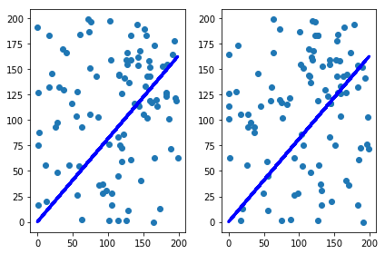
beta_x =  [[ 0.8158522]]  ; beta_y =  [[ 0.8158522]]