Exercise 3.13

%matplotlib inline
import numpy as np
import pandas as pd

import statsmodels.formula.api as smf
from sklearn.linear_model import LinearRegression

import matplotlib.pyplot as plt
import seaborn as sns


np.random.seed(1)
# does not generate the same sequences as R
# it seems there's no easy, elegant way of getting Python and R to generate the same random sequences
# http://stackoverflow.com/questions/22213298/creating-same-random-number-sequence-in-python-numpy-and-r

(a)

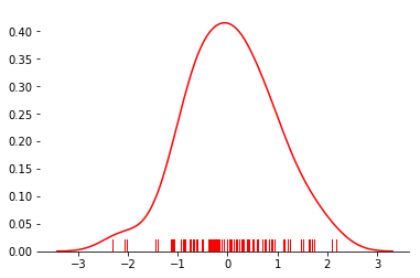
x = np.random.normal(size=100)

# http://seaborn.pydata.org/examples/distplot_options.html
fig, ax = plt.subplots()
sns.despine(left=True)

# Plot a kernel density estimate and rug plot
sns.distplot(x, hist=False, rug=True, color="r", ax=ax);

png

(b)

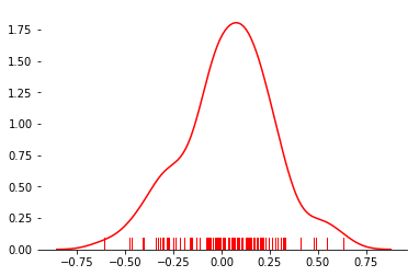
eps = np.random.normal(scale = .25, size=100)

fig, ax = plt.subplots()
sns.despine(left=True)
sns.distplot(eps, hist=False, rug=True, color="r", ax=ax);

png

(c)

y = -1 + .5*x + eps
print('Length of y = ' + str(len(y)))

Length of y = 100

Naturally, vector y has length 100, since it is a linear combination of 2 vectors of length 100.

In this model $\beta_0 = -1$ and $\beta_1=1/2$ .

(d)

df = pd.DataFrame({'x': x, 'y': y})
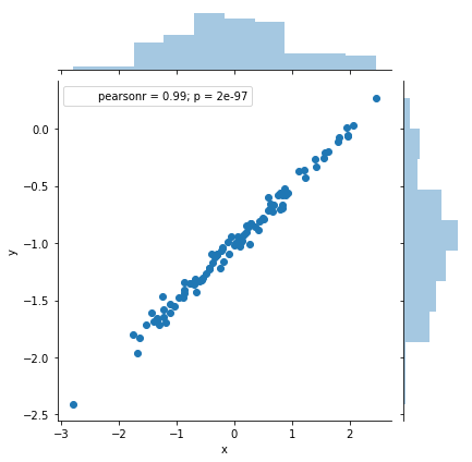
sns.jointplot(x='x', y='y', data=df);

png

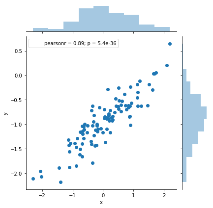
As expected, it does seem linear with a variance on the order of 0.5. No alarming indication of high leverage points or outliers.

(e)

reg = smf.ols('y ~ x', df).fit()
reg.summary()

OLS Regression Results
Dep. Variable:	y	R-squared:	0.800
Model:	OLS	Adj. R-squared:	0.798
Method:	Least Squares	F-statistic:	391.4
Date:	Fri, 08 Dec 2017	Prob (F-statistic):	5.39e-36
Time:	13:05:05	Log-Likelihood:	4.1908
No. Observations:	100	AIC:	-4.382
Df Residuals:	98	BIC:	0.8288
Df Model:	1
Covariance Type:	nonrobust

	coef	std err	t	P>\|t\|	[0.025	0.975]
Intercept	-0.9632	0.023	-40.999	0.000	-1.010	-0.917
x	0.5239	0.026	19.783	0.000	0.471	0.576

Omnibus:	0.898	Durbin-Watson:	2.157
Prob(Omnibus):	0.638	Jarque-Bera (JB):	0.561
Skew:	-0.172	Prob(JB):	0.755
Kurtosis:	3.127	Cond. No.	1.15

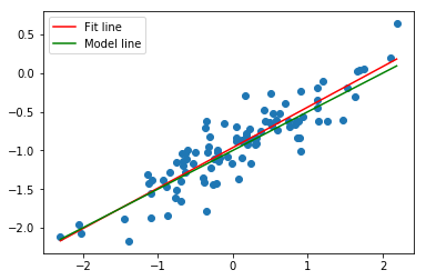
The coefficients of the regression are similar to the "true" values, although they are not equal (naturally). They fall within the 95% confidence interval in both cases.

(f)

model = LinearRegression(fit_intercept= True)
model.fit(x[:, np.newaxis],y)


plt.scatter(df.x, df.y);

xfit = np.linspace(df.x.min(), df.x.max(), 100)
yfit = model.predict(xfit[:, np.newaxis])
fit, = plt.plot(xfit, yfit, color='r');

xpop = np.linspace(df.x.min(), df.x.max(), 100)
ypop = -1 + .5*xpop
pop, = plt.plot(xpop, ypop, color='g');
plt.legend([fit, pop],['Fit line','Model line'])

<matplotlib.legend.Legend at 0x10c324eb8>

png

(g)

reg = smf.ols('y ~ x + I(x**2)', df).fit()
reg.summary()

OLS Regression Results
Dep. Variable:	y	R-squared:	0.800
Model:	OLS	Adj. R-squared:	0.796
Method:	Least Squares	F-statistic:	193.8
Date:	Fri, 08 Dec 2017	Prob (F-statistic):	1.32e-34
Time:	13:05:14	Log-Likelihood:	4.2077
No. Observations:	100	AIC:	-2.415
Df Residuals:	97	BIC:	5.400
Df Model:	2
Covariance Type:	nonrobust

	coef	std err	t	P>\|t\|	[0.025	0.975]
Intercept	-0.9663	0.029	-33.486	0.000	-1.024	-0.909
x	0.5234	0.027	19.582	0.000	0.470	0.576
I(x ** 2)	0.0039	0.021	0.181	0.856	-0.038	0.046

Omnibus:	0.893	Durbin-Watson:	2.152
Prob(Omnibus):	0.640	Jarque-Bera (JB):	0.552
Skew:	-0.170	Prob(JB):	0.759
Kurtosis:	3.132	Cond. No.	2.10

After fitting a model with basis functions $X$ and $X^2$ , looking at the table above we can see that the p-value for the squared term is 0.856, so we can conclude that there is no evidence to reject the null hypothesis asserting the coefficient of the second order term is zero. In other words, there is no statistically significant relationship between $X^2$ and $Y$ - the quadratic term does not improve the model fit. This is also evident when comparing the R-squared of both fits. They are equal, even though the second model has an additional variable.

(h)

x = np.random.normal(size=100)
eps = np.random.normal(scale = .05, size=100)
y = -1 + .5*x + eps

df = pd.DataFrame({'x': x, 'y': y})
sns.jointplot(x='x', y='y', data=df)

model = LinearRegression(fit_intercept= True)
model.fit(x[:, np.newaxis],y)

plt.subplots()
plt.scatter(df.x, df.y);


xfit = np.linspace(df.x.min(), df.x.max(), 100)
yfit = model.predict(xfit[:, np.newaxis])
fit, = plt.plot(xfit, yfit, color='r');

xpop = np.linspace(df.x.min(), df.x.max(), 100)
ypop = -1 + .5*xpop
pop, = plt.plot(xpop, ypop, color='g');
plt.legend([fit, pop],['Fit line','Model line'])

<matplotlib.legend.Legend at 0x10c742b38>

png

reg = smf.ols('y ~ x', df).fit()
reg.summary()

OLS Regression Results
Dep. Variable:	y	R-squared:	0.989
Model:	OLS	Adj. R-squared:	0.989
Method:	Least Squares	F-statistic:	8662.
Date:	Fri, 08 Dec 2017	Prob (F-statistic):	1.97e-97
Time:	13:05:22	Log-Likelihood:	151.58
No. Observations:	100	AIC:	-299.2
Df Residuals:	98	BIC:	-293.9
Df Model:	1
Covariance Type:	nonrobust

	coef	std err	t	P>\|t\|	[0.025	0.975]
Intercept	-1.0010	0.005	-186.443	0.000	-1.012	-0.990
x	0.4972	0.005	93.071	0.000	0.487	0.508

Omnibus:	0.426	Durbin-Watson:	1.977
Prob(Omnibus):	0.808	Jarque-Bera (JB):	0.121
Skew:	-0.045	Prob(JB):	0.941
Kurtosis:	3.145	Cond. No.	1.01

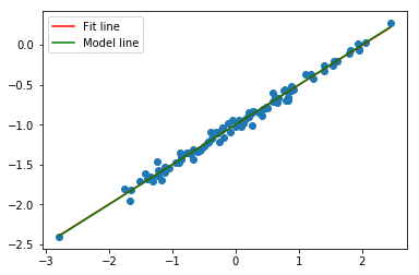
As expected, we have a better fit, a better confidence intervals, and a higher R-squared.

Our model fits this data set better than the previous one that was generated from a noisier distribution.

(i)

x = np.random.normal(size=100)
eps = np.random.normal(scale = 1, size=100)
y = -1 + .5*x + eps

df = pd.DataFrame({'x': x, 'y': y})
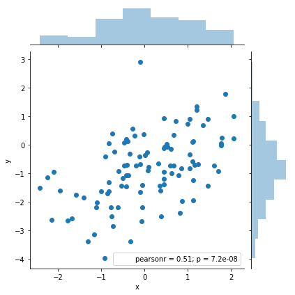
sns.jointplot(x='x', y='y', data=df)

model = LinearRegression(fit_intercept= True)
model.fit(x[:, np.newaxis],y)

plt.subplots()
plt.scatter(df.x, df.y);


xfit = np.linspace(df.x.min(), df.x.max(), 100)
yfit = model.predict(xfit[:, np.newaxis])
fit, = plt.plot(xfit, yfit, color='r');

xpop = np.linspace(df.x.min(), df.x.max(), 100)
ypop = -1 + .5*xpop
pop, = plt.plot(xpop, ypop, color='g');
plt.legend([fit, pop],['Fit line','Model line'])

<matplotlib.legend.Legend at 0x10bc05b00>

png

(i)

reg = smf.ols('y ~ x', df).fit()
reg.summary()

OLS Regression Results
Dep. Variable:	y	R-squared:	0.257
Model:	OLS	Adj. R-squared:	0.250
Method:	Least Squares	F-statistic:	33.96
Date:	Fri, 08 Dec 2017	Prob (F-statistic):	7.19e-08
Time:	13:05:27	Log-Likelihood:	-145.66
No. Observations:	100	AIC:	295.3
Df Residuals:	98	BIC:	300.5
Df Model:	1
Covariance Type:	nonrobust

	coef	std err	t	P>\|t\|	[0.025	0.975]
Intercept	-0.8802	0.105	-8.375	0.000	-1.089	-0.672
x	0.5903	0.101	5.828	0.000	0.389	0.791

Omnibus:	3.633	Durbin-Watson:	1.972
Prob(Omnibus):	0.163	Jarque-Bera (JB):	3.566
Skew:	0.192	Prob(JB):	0.168
Kurtosis:	3.842	Cond. No.	1.07

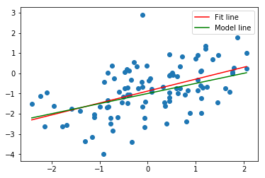
Now, on the other hand, we have a much worse fit. The R-squared is just .178 and the confidence intervals for the coefficients are much wider. Still there's no doubt we are in the presence of a statistically significant relationship, with very low p-values.

(j)

Here's a table with the various confidence intervals:

Noise	lower $\beta_0$	$\beta_0$	upper $\beta_0$	lower $\beta_1$	$\beta_1$	upper $\beta_1$
$\varepsilon = .05$	-1.009	0.9984	-0.987	0.489	0.5002	0.512
$\varepsilon=.25$	-1.010	-0.9632	-0.917	0.471	0.5239	0.576
$\varepsilon = 1$	-1.098	-0.8869	-0.675	0.267	0.4697	0.672

As expected the width of the intervals increases as the level of noise increases.